Mixed Effect Machine Learning (Journal Club)

Mahidol University, Thailand 19 March 2021

I presdented at a journal club regarding the topic of “Mixed Effect Machine Learning”. The presentation was based on the paper by Che Ngufora, Holly Van Houten, Brian S. Caffo, Nilay D. Shah and Rozalina G. McCoy, published in Journal of Biomedical Informatics (2018). The resources for the Journal Club can be found here.

The Challenge of Correlated Observations

Traditional machine learning algorithms rely heavily on the assumption that data points are Independent and Identically Distributed (i.i.d). However, this assumption is often violated in clinical data:

Clustered data: such as patients treated within the same hospital or students in classrooms.
Longitudinal data: where repeated measures are taken from the same subject over time.

This correlation results in a loss of independence. Classical machine learning models applied directly to such data often fail to generate high-quality, generalizable predictions.

Mixed Effects Models Overview

To account for these correlations, statisticians traditionally use Mixed Effects Models.

Linear Mixed Model

The traditional Linear Mixed Model separates the effects into two components:

$$ y_{ij} = X_{ij}b + Z_{ij}u $$

Where:

**$y$ is the target variable.
$X_{ij}b$ is the population-average value (Fixed Effects), accounting for within-cluster variation.
$Z_{ij}u$ is the subject-specific value (Random Effects), accounting for between-cluster variation.

Non-linear Mixed Model

This concept extends to non-linear relationships:

$$ y_{ij} = f(X_{ij}) + Z_{ij}u $$

Here, $f(x)$ is a non-linear function representing the fixed effects.

The Mixed Effect Machine Learning Framework

The core innovation of the paper is replacing the traditional non-linear function $f(x)$ with a machine learning regressor (such as Random Forest or Gradient Boosting Machines):

$$ y = f_{ML}(x) + Zu $$

In this framework, the random effect (RE) is considered the intra-subject or intra-cluster variability. The core methodology aims to mathematically exclude this RE from the total effect. By subtracting the RE, the resulting modified target consists of non-correlated observations lacking intra-cluster variability. Training the machine learning (or non-linear classifier) model on this remaining, independent fixed effect is the primary goal.

The model learns these two components separately through an iterative Expectation-Maximization (EM) like algorithm:

Fixed effects are estimated using machine learning methods.
Random effects are estimated using linear mixed models.

Training via Expectation-Maximization

The training process uses an iterative Expectation-Maximization (EM) like algorithm. The standard EM algorithm handles incomplete data by alternating between two steps until convergence:

Expectation Step (E-step): Uses the currently available data and parameter estimates to guess the values of the “missing” or latent data.
Maximization Step (M-step): Uses that complete data (observed + guessed) to update the parameters and maximize the model’s likelihood.

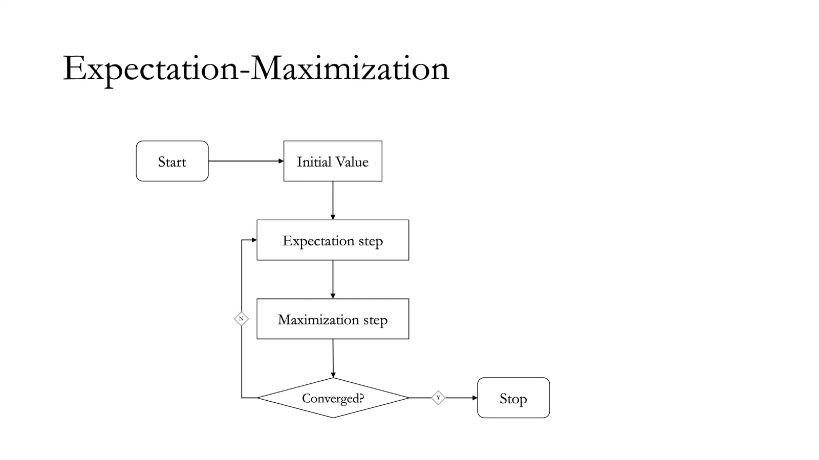
Figure 1. The EM algorithm iteratively estimates the missing data and updates the model parameters until convergence. In the context of Mixed Effects Machine Learning, the “missing” data are the isolated fixed and random effects, which must be iteratively estimated.

IterativeImputator from scikit-learn is an example of an EM-like algorithm that iteratively imputes missing values. In the context of Mixed Effects Machine Learning, the “missing” data are the isolated fixed and random effects, which must be iteratively estimated.

Continuous Target (Regression)

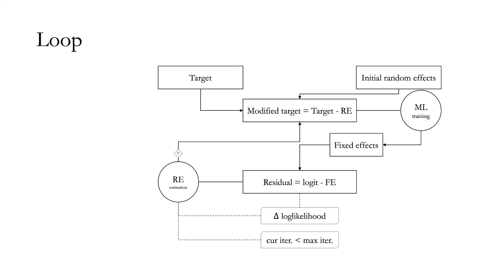
For continuous targets, the model is trained using a single iterative loop as shown in Figure 2:

Start with an initial guess for the random effects.
Modify the target: Subtract the current random effects from the actual target.
Train the ML model: Fit the machine learning regressor on this modified target to estimate the fixed effects.
Calculate residuals: Subtract the fixed effects from the original target.
Estimate Random Effects: Fit a Linear Mixed Model on these residuals.
Check for convergence: Calculate the change in log-likelihood. If the change is below a set tolerance or the maximum iterations are reached, stop. Otherwise, update the random effects and repeat from step 2.

Figure 2. The goal is to exclude the random effects from the target variable, allowing the machine learning model to focus on learning the fixed effects. The modified target lacking the random effects is considered to be independent and identically distributed (i.i.d), making it suitable for training the machine learning model.

Binary Target (Classification)

For binary classification tasks, the framework employs a nested loop structure. Unlike regression where the continuous target is directly modified, classification requires estimating the underlying continuous logit (log-odds) values. Since the true logit values are unknown and must be iteratively approximated, a double loop is necessary: an inner loop to fit the model to the current logit estimates (similar to the regression loop), and an outer loop to update those logit estimates.

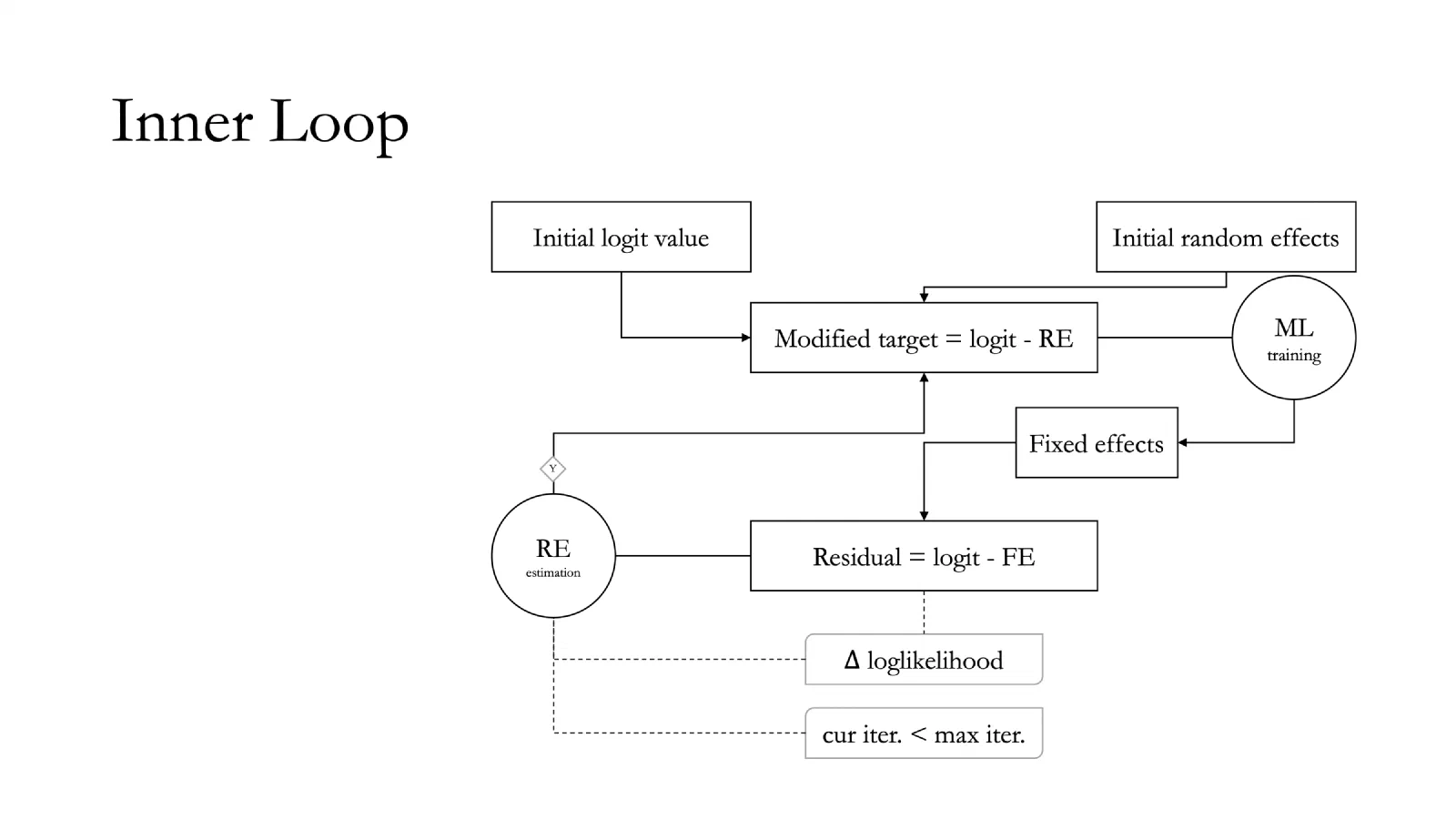
Inner Loop:

This loop functions similarly to the regression loop but operates on the current estimated logit values rather than the raw target as presented in Figure 3:

Modify the target: Subtract the current random effects from the current logit value.
Train the ML model: Fit the machine learning regressor on this modified target to estimate the fixed effects (FE).
Calculate residuals: Subtract the fixed effects from the current logit value.
Estimate Random Effects: Fit a Linear Mixed Model on these residuals to estimate the random effects (RE).
Check for Inner Convergence: Calculate the change in log-likelihood. If the change is below a set tolerance, stop and return the FE and RE to the Outer Loop. Otherwise, update the random effects and repeat the Inner Loop.

Figure 3. The inner loop focuses on refining the estimates of fixed and random effects for the current logit values. By iteratively updating these estimates, the model can effectively capture the underlying structure of the data, leading to improved classification performance.

Outer Loop:

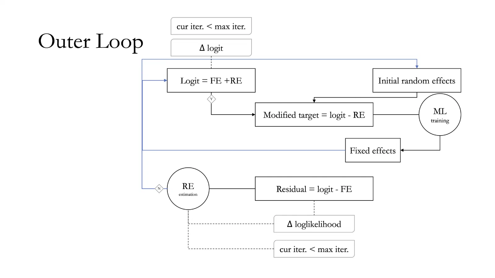
As it is observed in Figure 4, this loop governs the overall process by updating the overall logit values based on the inner loop’s output.

Initialize the logit values based on the target class probabilities.
Initialize random effects.
Run the Inner Loop to convergence (or max iterations) to find the best Fixed Effects (FE) and Random Effects (RE) for the current logit values.
Update Logit Values: Calculate the new logit values: $\text{Logit} = FE + RE$.
Check for Outer Convergence: Evaluate the absolute change in the logit value ($\Delta \text{logit}$). If the change is below the tolerance limit, stop. Otherwise, repeat the Outer Loop with the newly calculated logit values.

Figure 4. The outer loop iteratively updates the logit values based on the estimated fixed and random effects from the inner loop. The inner loop focuses on refining the estimates of FE and RE for the current logit values, while the outer loop ensures that these estimates converge to a stable solution.

Results and Implications

The authors demonstrated significant improvements when using Mixed Effects Machine Learning over classical machine learning methods on clustered/longitudinal data.

As the number of repeated observations increased, the performance of the mixed-effects ML approach improved, whereas classical methods deteriorated.
By incorporating random effects, the models became resistant to variabilities introduced by correlated data and could leverage those dependencies to generate more robust predictions.
Note: While superior to basic ML, the paper noted that an improvement over generalized linear mixed models (GLMM) was not necessarily observed.

Documents

The paper is available here, and mirrored here. I served as the presentation lead, and the presentation slides are available here. Mr Pongsathorn Piebpien served as the commentator, and his commentary slides are available here.

Practical Application

Later, I applied this framework as one of the models in my research. The model application is detailed in:

The corresponding journal manuscript was eventually published in JMIR Formative Research (2023).